The dangers of overfitting: a Kaggle postmortem
July 06, 2012
Over the last month and a half, the Online Privacy Foundation hosted a Kaggle competition, in which competitors attempted to predict the psychopathy levels of Twitter users. The bigger goal here is to learn how much of our personality is actually revealed through services like Twitter, and by hosting on Kaggle, the Online Privacy Foundation can sit back and watch competitors squeeze every bit of information out of the data.
Competitors can submit two sets of predictions each day, and each submission is scored from 0 (worst) to 1 (best) using a metric known as average precision. Essentially, a submission that predicts the correct ranking of psychopathy scores across all Twitter accounts will receive an average precision score of 1.
I made 42 submissions, making it my biggest Kaggle effort yet. Each submission is instantly scored, and competitors are ranked on a public leaderboard by their best submission. However, the public leaderboard score isn’t actually the true score—it is only an estimate based on a small portion of the submission. When the competition ends, five submissions from each competitor are compared to the full set of test data, and the highest scoring submission from each user is used to calculate the final score. By the end of the contest, I had slowly worked my way up to 2nd place on the public leaderboard, shown below.
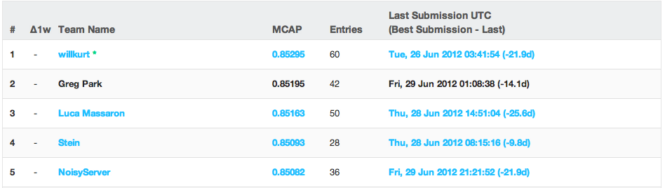 Top of the public leaderboard. The public leaderboard scores are calculated during the competition by comparing users’ predictions to a small subset of the test data.
I held this spot for the last week and felt confident that I would maintain a decent spot on the private, or true, leaderboard. Soon after the competition closed, the private leaderboard was revealed. Here’s what I saw at the top:
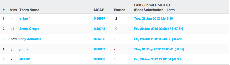 Top of the private leaderboard. The private leaderboard is the “real” leaderboard, revealed after the contest is closed. Scores are calculated by comparing users’ predictions to the full set of test data.
Where’d I go? I scrolled down the leaderboard…. further… and further… and finally found my name:
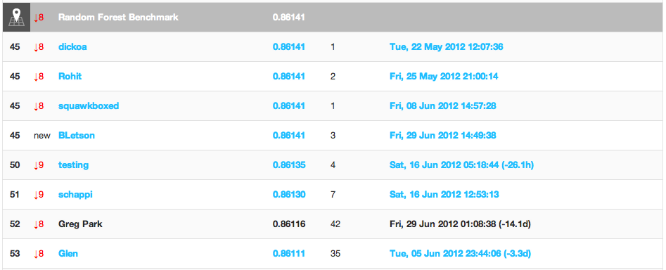 My place on the private leaderboard. I dropped from 2nd place on the public leaderboard to 52nd on the private leaderboard. Notice I placed below the random forest benchmark!
Somehow I managed to fall from 2nd all the way down to 52nd! I wasn’t the only one who took a big fall: the top five users on the public leaderboard ended up in 64th, 52nd, 58th, 16th, and 57th on the private leaderboard, respectively. I even placed below the random forest benchmark, a solution publicly available from the start of the competition.
What happened?
After getting over the initial shock of dropping 50 places, I began sifting through the ashes to figure out what went so wrong. I think those with more experience already know, but one clue is in the screenshot of the pack leaders on the public leaderboard. Notice that the top five users, including myself, have a lot of submissions. For context, the median number of submissions in this contest was six. Contrast this with the (real) leaders on the private leaderboard – most have less than 12 submissions. Below, I’ve plotted the number of entries from each user against their final standing on the public and private leaderboards and added a trend line to each plot.
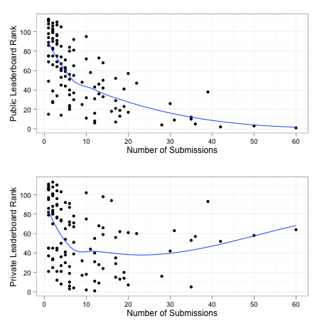
On the public leaderboard, more submissions are consistently related to a better standing. It could be that the public leaderboard actually reflects the amount of brute force from a competitor rather than predictive accuracy. If you throw enough mud at a wall, eventually some of it will start to stick. The problem is that submissions that score well using this approach probably will not generalize to the full set of test data when the competition closes. It’s possible to overfit the portion of test data used to calculate the public leaderboard, and it looks like that’s exactly what I did.
Compare that trend in the public leaderboard to the U-shaped curve in the plot of the private leaderboard and number of submissions. After about 25 submissions or so, private leaderboard standings get worse with the number of submissions.
Poor judgments under uncertainty
Overfitting the public leaderboard is not unheard of, and I knew that it was a possibility all along. So why did I continue to hammer away at competition with so many submissions, knowing that I could be slowly overfitting to the leaderboard?
Many competitors with estimate the quality of their submissions prior to uploading them using cross-validation. Because the public leaderboard is only based on a small portion of the test data, it is only a rough estimate of the true quality of a submission, and cross-validation gives a sort of second opinion of a submission’s quality. For most of my submissions, I used 10-fold cross-validation to estimate the average precision. So throughout the contest, I could observe both the public leaderboard score and my own estimated score from cross-validation. After the contest closes, Kaggle reveals the private or true score of each submission. Below, I’ve plotted the public, private, and cv-estimated score of each submission by date. The dotted line is the private score of the winning submission.
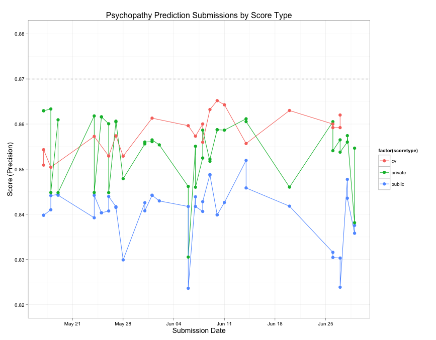
There are a few things worth pointing out here:
- My cross-validation (CV) estimated scores (the orange line) gradually improve over time. So, as far as I know, my submissions are actually getting better as I go.
- The private or true scores actually get worse over time. In fact, my first two submissions to the contest turned out to be my best (and I did not choose them as any of my final five submissions)
- The public scores reach a peak and then slowly get worse at the end of the contest.
- It is very difficult to see a relationship between any of these trends.
Below, I’ve replaced the choppy lines with smoothed lines to show the general trends.
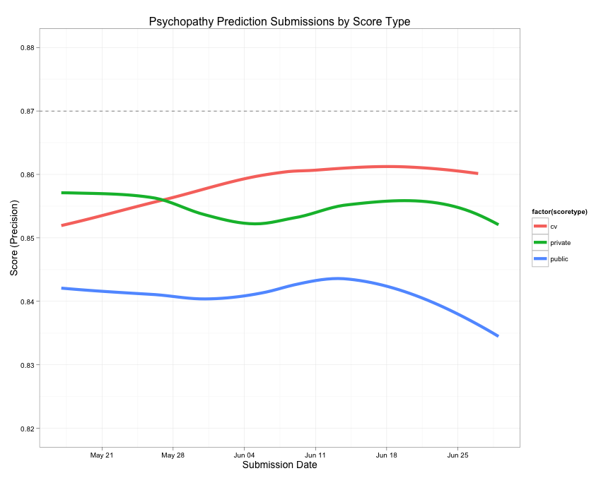 An alternate plot of the submission scores over time using smoothers to depict some general trends.
Based on my experience with past contests, I knew that the public leaderboard could not be trusted fully, and this is why I used cross-validation. I assumed that there was a stronger relationship between the cross-validation estimates and the private leaderboard than between the public and private leaderboard. Below, I’ve created scatterplots to show the relationships between each pair of score types.
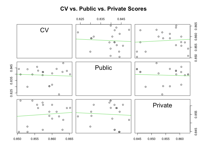 Scatterplots of three types of scores for each submission: 10-fold CV estimated score, public leaderboard score, and private or “true” score.
The scatterplots tell a different story. It turned out that my cross-validation estimates were not related to the private scores at all (notice the horizontal linear trends in those scatterplots), and the public leaderboard wasn’t any better. I already guessed that the public leaderboard would be a poor estimate of the true score, but why didn’t cross-validation do any better?
I suspect this is because as the competition went on, I began to use much more feature selection and preprocessing. However, I made the classic mistake in my cross-validation method by not including this in the cross-validation folds (for more on this mistake, see this short description or section 7.10.2 in The Elements of Statistical Learning). This lead to increasingly optimistic cross-validation estimates. I should have known better, but under such uncertainty, I fooled myself into accepting the most self-serving description of my current state. Even worse, I knew not to trust the public leaderboard, but when I started to edge towards to the top, I began to trust it again!
Lessons learned
In the end, my slow climb up the leaderboard was due mostly to luck. I chose my five final submissions based on cross-validation estimates, which turned out to be a poor predictor of true score. Ultimately, I did not include my best submissions in the final five, which would have brought me up to 33rd place – not all that much better than 52nd. All said, this was my most educational Kaggle contest yet. Here are some things I’ll take into the next contest:
- It is easier to overfit the public leaderboard than previously thought. Be more selective with submissions.
- On a related note, perform cross-validation the right way: include all training (feature selection, preprocessing, etc.) in each fold.
- Try to ignore the public leaderboard, even when it is telling you nice things about yourself.
Some sample code
One of my best submissions (average precision = .86294) was actually one of my own benchmarks that took very little thought. By stacking this with two other models (random forests and elastic net), I was able to get it up to .86334 (edit: and yes, those tiny little increases actually make a difference on the leaderboard!). Since the single model is pretty simple, I’ve included the code. After imputing missing values in the training and test set with medians, I used the gbm package in R to fit a boosting model using every column in the data as predictor. The hyperparameters were not tuned at all, just some reasonable starting values. I used the internal cross-validation feature of gbm to choose the number of trees. The full code from start to finish is below:
  library(gbm)

  # impute.NA is a little function that fills in NAs with either means or medians
impute.NA <- function(x, fill="mean"){
  if (fill=="mean")
  {
    x.complete <- ifelse(is.na(x), mean(x, na.rm=TRUE), x)
  }

  if (fill=="median")
  {
    x.complete <- ifelse(is.na(x), median(x, na.rm=TRUE), x)
  }

  return(x.complete)
}

data <- read.table("Psychopath_Trainingset_v1.csv", header=T, sep=",")
testdata <- read.table("Psychopath_Testset_v1.csv", header=T, sep=",")

# Median impute all missing values
# Missing values are in columns 3-339
fulldata <- apply(data[,3:339], 2, FUN=impute.NA, fill="median")
data[,3:339] <- fulldata

fulltestdata <- apply(testdata[,3:339], 2, FUN=impute.NA, fill="median")
testdata[,3:339] <- fulltestdata

# Fit a generalized boosting model

# Create a formula that specifies that psychopathy is to be predicted using
# all other variables (columns 3-339) in the dataframe

gbm.psych.form <- as.formula(paste("psychopathy ~",
                                   paste(names(data)[c(3:339)], collapse=" + ")))

# Fit the model by supplying gbm with the formula from above.
# Including the train.fraction and cv.folds argument will perform
# cross-validation

gbm.psych.bm.1 <- gbm(gbm.psych.form, n.trees=5000, data=data,
                      distribution="gaussian", interaction.depth=6,
                      train.fraction=.8, cv.folds=5)

# gbm.perf will return the optimal number of trees to use based on
# cross-validation. Although I grew 5,000 trees, cross-validation suggests that
# the optimal number of trees is about 4,332.

best.cv.iter <- gbm.perf(gbm.psych.bm.1, method="cv") # 4332

# Use the trained model to predict psychopathy from the test data.

gbm.psych.1.preds <- predict(gbm.psych.bm.1, newdata=testdata, best.cv.iter)

# Package it in a dataframe and write it to a .csv file for uploading.

gbm.psych.1.bm.preds <- data.frame(cbind(myID=testdata$myID,
                                         psychopathy=gbm.psych.1.preds))

write.table(gbm.psych.1.bm.preds, "gbmbm1.csv", sep=",", row.names=FALSE)
An earlier verison of this post appeared on Kaggle’s blog: No Free Hunch here